Gram-Schmidt Process in Plane and Space: Visual Orthonormalization

The Story: Building an Orthonormal World from Arbitrary Directions

The Gram-Schmidt Process is an algorithm for orthonormalizing a set of vectors in an inner product space. But before diving into formulas, let’s explain what this algorithm does.

If you are handed an arbitrary, skewed set of coordinate axes that span a space, how do you straighten them out into a pristine set of mutually perpendicular, unit-length grid lines—without altering the space they enclose?

---

1. Perpendicularity Relationship between Lines in Space

In geometry, one of the primary relationships between two lines in space is perpendicularity. We say that one line is perpendicular to another line if the first line meets the second line at right angles ($90^\circ$).

Perpendicularity is a symmetric relationship:

$$ L_1 \perp L_2 \iff L_2 \perp L_1 $$

In other words, if one line is perpendicular to the second line, the second line is also perpendicular to the first line. Therefore, you can say that two lines are perpendicular to each other or the two lines are mutually perpendicular.

---

2. Orthogonality Relationship between Vectors in an Inner Product Space

In linear algebra, one of the primary relationships between two vectors is orthogonality. You can think of the orthogonality relationship between two vectors in an inner product space as a generalization of the perpendicularity relationship between two lines in geometry space.

We say that vector $\mathbf{u}$ is orthogonal to vector $\mathbf{v}$ in an inner product space if the inner product equals zero:

$$ \langle \mathbf{u}, \mathbf{v} \rangle = 0 $$

(In standard Euclidean space $\mathbb{R}^n$, the inner product is the familiar dot product: $\mathbf{u} \cdot \mathbf{v} = 0$.)

Since the inner product is symmetric ($\langle \mathbf{u}, \mathbf{v} \rangle = \langle \mathbf{v}, \mathbf{u} \rangle$), if one vector is orthogonal to the second vector, the second vector is also orthogonal to the first vector:

$$ \mathbf{u} \perp \mathbf{v} \iff \mathbf{v} \perp \mathbf{u} $$

Therefore, you can say that two vectors are orthogonal to each other or the two vectors are orthogonal.

---

3. Orthonormalizing Vectors in an Inner Product Space

We say that a set of vectors is orthogonal if each pair of distinct vectors in the set is orthogonal:

$$ \langle \mathbf{u}_i, \mathbf{u}_j \rangle = 0 \quad \text{for all } i \neq j $$

When we orthonormalize vectors in an inner product space, we take a set of vectors that should be linearly independent and finite, and generate a new set of vectors that is orthogonal and spans the original set:

$$ \text{span}\{\mathbf{u}_1, \dots, \mathbf{u}_k\} = \text{span}\{\mathbf{v}_1, \dots, \mathbf{v}_k\} $$

In other words, the purpose of the Gram-Schmidt Process is to generate a new set of vectors that is orthogonal and spans the input set of the algorithm.

---

Part 1: The Process in the Plane ($\mathbb{R}^2$)

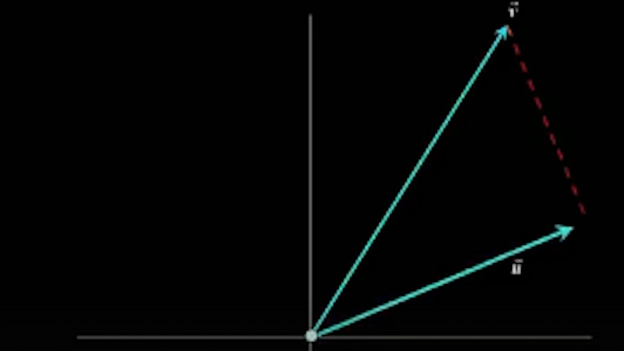
In two dimensions, we start with two linearly independent vectors $\mathbf{v}_1$ and $\mathbf{v}_2$:

1. Step 1 — Choose the First Anchor: Pick the first vector as our reference direction:

   $$\mathbf{u}_1 = \mathbf{v}_1$$

2. Step 2 — Decompose the Second Vector: The vector $\mathbf{v}_2$ decomposes into two perpendicular components: a component parallel to $\mathbf{u}_1$, and a component perpendicular to $\mathbf{u}_1$:

   $$\mathbf{v}_2 = \text{proj}_{\mathbf{u}_1}(\mathbf{v}_2) + \mathbf{u}_2$$

3. Step 3 — Subtract the Projection: Using the orthogonal projection formula $\text{proj}_{\mathbf{u}_1}(\mathbf{v}_2) = \frac{\langle \mathbf{v}_2, \mathbf{u}_1 \rangle}{\langle \mathbf{u}_1, \mathbf{u}_1 \rangle} \mathbf{u}_1$, we isolate the orthogonal vector $\mathbf{u}_2$:

   $$\mathbf{u}_2 = \mathbf{v}_2 - \frac{\langle \mathbf{v}_2, \mathbf{u}_1 \rangle}{\langle \mathbf{u}_1, \mathbf{u}_1 \rangle} \mathbf{u}_1$$

Now $\{\mathbf{u}_1, \mathbf{u}_2\}$ forms an orthogonal basis for the 2D plane!

---

Part 2: Extending into Space ($\mathbb{R}^3$)

In three-dimensional space, we introduce a third linearly independent vector $\mathbf{v}_3$.

Vectors $\mathbf{u}_1$ and $\mathbf{u}_2$ already define a 2D orthogonal floor. Vector $\mathbf{v}_3$ points into 3D space, but may have non-zero components along both $\mathbf{u}_1$ and $\mathbf{u}_2$.

To make $\mathbf{u}_3$ strictly perpendicular to the entire floor:

1. Compute the projection of $\mathbf{v}_3$ onto $\mathbf{u}_1$.
2. Compute the projection of $\mathbf{v}_3$ onto $\mathbf{u}_2$.
3. Subtract both projections simultaneously from $\mathbf{v}_3$:

$$ \mathbf{u}_3 = \mathbf{v}_3 - \text{proj}_{\mathbf{u}_1}(\mathbf{v}_3) - \text{proj}_{\mathbf{u}_2}(\mathbf{v}_3) $$$$ \mathbf{u}_3 = \mathbf{v}_3 - \frac{\langle \mathbf{v}_3, \mathbf{u}_1 \rangle}{\langle \mathbf{u}_1, \mathbf{u}_1 \rangle} \mathbf{u}_1 - \frac{\langle \mathbf{v}_3, \mathbf{u}_2 \rangle}{\langle \mathbf{u}_2, \mathbf{u}_2 \rangle} \mathbf{u}_2 $$

Now $\mathbf{u}_3 \perp \mathbf{u}_1$ and $\mathbf{u}_3 \perp \mathbf{u}_2$. The triad $\{\mathbf{u}_1, \mathbf{u}_2, \mathbf{u}_3\}$ is completely mutually orthogonal in 3D!

---

Final Step: Normalization (From Orthogonal to Orthonormal)

Once all vectors are mutually perpendicular, we normalize each vector by dividing by its magnitude (norm):

$$ \mathbf{e}_1 = \frac{\mathbf{u}_1}{\|\mathbf{u}_1\|}, \quad \mathbf{e}_2 = \frac{\mathbf{u}_2}{\|\mathbf{u}_2\|}, \quad \mathbf{e}_3 = \frac{\mathbf{u}_3}{\|\mathbf{u}_3\|} $$

The resulting set $\{\mathbf{e}_1, \mathbf{e}_2, \mathbf{e}_3\}$ is an orthonormal basis of $\mathbb{R}^3$.

---

Summary: The General Gram-Schmidt Formula

For any finite linearly independent set $\{\mathbf{v}_1, \mathbf{v}_2, \dots, \mathbf{v}_k\}$ in an inner product space:

$$ \mathbf{u}_1 = \mathbf{v}_1 $$$$ \mathbf{u}_k = \mathbf{v}_k - \sum_{j=1}^{k-1} \frac{\langle \mathbf{v}_k, \mathbf{u}_j \rangle}{\langle \mathbf{u}_j, \mathbf{u}_j \rangle} \mathbf{u}_j $$$$ \mathbf{e}_k = \frac{\mathbf{u}_k}{\|\mathbf{u}_k\|} $$

Why Are Orthonormal Bases So Essential?

1. Effortless Coordinates: Finding the coordinates of any arbitrary vector $\mathbf{x}$ requires no matrix inversion—simply compute dot products: $\mathbf{x} = \sum_{i=1}^k \langle \mathbf{x}, \mathbf{e}_i \rangle \mathbf{e}_i$.
2. Numerical Stability: In computer graphics, signal processing, and machine learning, orthonormal transformations preserve distances, angles, and avoid matrix condition number degradation ($QR$ decomposition).